Basic Image processing using PIL and Opencv
by Hasan
Here we will see very basic image processing steps using two useful libraries.
- PIL
- Opencv
Both libraries provides us very similar functionlity.
Getting image
here I am using jupyter notebook. In jupyter notebook you can use bash command line using ! sign. In the following line I am telling with wget command, that please go to link and save image. After that -O says that output, that means output link. I have used only name, so the images will be saved in my current directory using the name I have provided after -O
!wget https://cf-courses-data.s3.us.cloud-object-storage.appdomain.cloud/IBMDeveloperSkillsNetwork-CV0101EN-SkillsNetwork/images%20/images_part_1/lenna.png -O lenna.png
!wget https://cf-courses-data.s3.us.cloud-object-storage.appdomain.cloud/IBMDeveloperSkillsNetwork-CV0101EN-SkillsNetwork/images%20/images_part_1/baboon.png -O baboon.png
!wget https://cf-courses-data.s3.us.cloud-object-storage.appdomain.cloud/IBMDeveloperSkillsNetwork-CV0101EN-SkillsNetwork/images%20/images_part_1/barbara.png -O barbara.png
--2021-08-10 19:41:44--  https://cf-courses-data.s3.us.cloud-object-storage.appdomain.cloud/IBMDeveloperSkillsNetwork-CV0101EN-SkillsNetwork/images%20/images_part_1/lenna.png
Resolving cf-courses-data.s3.us.cloud-object-storage.appdomain.cloud (cf-courses-data.s3.us.cloud-object-storage.appdomain.cloud)... 169.63.118.104
Connecting to cf-courses-data.s3.us.cloud-object-storage.appdomain.cloud (cf-courses-data.s3.us.cloud-object-storage.appdomain.cloud)|169.63.118.104|:443... connected.
HTTP request sent, awaiting response... 200 OK
Length: 473831 (463K) [image/png]
Saving to: 'lenna.png’

lenna.png           100%[===================>] 462,73K   859KB/s    in 0,5s

2021-08-10 19:41:47 (859 KB/s) - 'lenna.png’ saved [473831/473831]

--2021-08-10 19:41:47--  https://cf-courses-data.s3.us.cloud-object-storage.appdomain.cloud/IBMDeveloperSkillsNetwork-CV0101EN-SkillsNetwork/images%20/images_part_1/baboon.png
Resolving cf-courses-data.s3.us.cloud-object-storage.appdomain.cloud (cf-courses-data.s3.us.cloud-object-storage.appdomain.cloud)... 169.63.118.104
Connecting to cf-courses-data.s3.us.cloud-object-storage.appdomain.cloud (cf-courses-data.s3.us.cloud-object-storage.appdomain.cloud)|169.63.118.104|:443... connected.
HTTP request sent, awaiting response... 200 OK
Length: 637192 (622K) [image/png]
Saving to: 'baboon.png’

baboon.png          100%[===================>] 622,26K   884KB/s    in 0,7s

2021-08-10 19:41:49 (884 KB/s) - 'baboon.png’ saved [637192/637192]

--2021-08-10 19:41:49--  https://cf-courses-data.s3.us.cloud-object-storage.appdomain.cloud/IBMDeveloperSkillsNetwork-CV0101EN-SkillsNetwork/images%20/images_part_1/barbara.png
Resolving cf-courses-data.s3.us.cloud-object-storage.appdomain.cloud (cf-courses-data.s3.us.cloud-object-storage.appdomain.cloud)... 169.63.118.104
Connecting to cf-courses-data.s3.us.cloud-object-storage.appdomain.cloud (cf-courses-data.s3.us.cloud-object-storage.appdomain.cloud)|169.63.118.104|:443... connected.
HTTy request sent, awaiting response... 200 OK
Length: 185727 (181K) [image/png]
Saving to: 'barbara.png’

barbara.png         100%[===================>] 181,37K   452KB/s    in 0,4s

2021-08-10 19:41:50 (452 KB/s) - 'barbara.png’ saved [185727/185727]
Image Files and paths
from pathlib import Path
import matplotlib.pyplot as plt

# Function to see all files in a directory.
# Stolen from fastai. :)
Path.ls = lambda x:sorted(list(x.iterdir()))
% matplotlib inline
% load_ext autoreload
% autoreload 2
my_image = 'lenna.png'
image_path = Path(Path.cwd()/my_image)
image_path
PosixPath('/home/hasan/Schreibtisch/projects/coursera/computer_vision_basic/lenna.png')
PIL image
from PIL import Image
# Just opening image to see it in jupyter notebook.
pil_image = Image.open(my_image)
# At first I want to see the type
type(pil_image)
PIL.PngImagePlugin.PngImageFile
# If we use the name, we can see it in jupyter notebook.Sometimes show method needs to be used. However with magic comman matplotlib inline, it is taken care.
pil_image

OpenCV
# Importing open cv library to use it
import cv2
# Reading image using opencv
cv_image = cv2.imread(my_image)
# Let see the type of the image
type(cv_image)
numpy.ndarray
The type is a numpy array.
- The value of
8bit unsigned Integer. - flag parmaters for
imreadis used to clarify how image should be read. defaultcv2.IMREAD_COLOR
cv_image.shape
(512, 512, 3)
cv_image.max(), cv_image.min()
(255, 3)
Important information
- Normally the intensity value is limited from 0 to 255
PILimage normally return pil array andopencvreturn numpy array. we can actually convert PIL image into numpy array easily. We will do it later.- PIL return
R, G, Bformat and opencv returns normallyB, G, Rformat
Plotting an image
PIL
We can use image.show or matplotlib function to show an image. When we use Image.open it doesnot load the image in computer memory, to load the image we need to use image.load method
pil_image.show()
In jupyter notebook this comman will creat another window with the image. Actually if we want to see the image, we just write the name of the image(in PIL), otherwise we can use matplotlib function, which will be same for both PIL and opencv.
Now we can do this using matplotlib function
fig, ax = plt.subplots(figsize=(10, 10))
ax.imshow(pil_image)
ax.axis('off')
(-0.5, 511.5, 511.5, -0.5)

We can see the mode of the image
pil_image.mode
'RGB'
Size of the images can also be seen using size
pil_image.size
(512, 512)
As we have said Image.open doesnot load it in memory. We are loading the image using load
pil_image_ar = pil_image.load()
type(pil_image_ar)
PixelAccess
Now it is loaded in memory, we can now index them as normal array
pil_image_ar[0, 1]
(226, 137, 125)
Saving can be done using normal save method
# pil_image.save('lena.png')
Opencv
# cv2.imshow() # can be done, another window will show up , therefore for jupyter notebook, we will be using matplotlib
fig, ax = plt.subplots(figsize=(10, 10))
ax.imshow(cv_image)
ax.axis('off')
(-0.5, 511.5, 511.5, -0.5)

As we can see, it is not the image, we are expecting. It is somehow difference, because of channel. As we said earlier opencv uses B, G, R format. and we need R, G, B image. It is not so difficult to convert it to R, G, B image
new_cv_image = cv2.cvtColor(cv_image, cv2.COLOR_BGR2RGB)
Another thing we can do, as we are repeating the matplotlib 3 lines. So we can just create a small fuction to use it in future.
def show_image(im, cmap=None):
    """
    show an image using matplotlib
    im:image
    """
    fig, ax = plt.subplots(figsize=(10, 10))
    ax.imshow(im,cmap=cmap)
    ax.axis('off')
Let’s see whether our function works or not
show_image(new_cv_image)

We can actually save the image
# cv2.imwrite('lenna.jpg', new_cv_image)
Grayscale Images
PIL
We now need anther module from PIL library, which is ImageOps for our further work
from PIL import ImageOps
pil_image_gray = ImageOps.grayscale(pil_image)
pil_image_gray

pil_image_gray.mode
'L'
L means gray scale image in PIL image library
Opencv
We can use both images, one image was the loaded image or the image we already have converted to rgb first. I guess it is better to use the image, which is saved in locally. However the function name will be changed. I have used both functions ( one is commented out)
cv_gray_image = cv2.cvtColor(new_cv_image, cv2.COLOR_RGB2GRAY)
# cv_gray_image = cv2.cvtColor(cv_image, cv2.COLOR_BGR2GRAY)
show_image(cv_gray_image, cmap='gray')

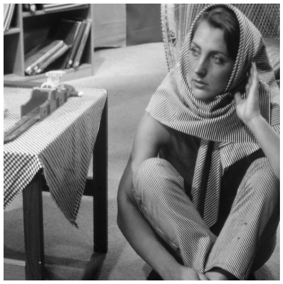
When loading a gray scale image, we need to change the flag, in case of opencv because default flg is cv2.IMREAD_COLOR, in case of gray scale we need to use cv2.IMREAD_GRAYSCALE flag
im_gray = cv2.imread('barbara.png', cv2.IMREAD_GRAYSCALE)
show_image(im_gray, cmap='gray')
Quantization PIL
- quantization is the number of pixel value, an image can take
- Normally images value ranges from
0 to 255 - We can change them, in pil image there is function called
quantize
pil_image_gray.quantize(256 // 2)

I want to see main image and quanized image side, therefore creating another function to see the effect clearly
def get_concat_h(im1,
                 im2):
    """
    two side by side images together
    """
    dst = Image.new('RGB', (im1.width  + im2.width, im1.height))
    dst.paste(im1, (0, 0))
    dst.paste(im2, (im1.width, 0))
    return dst
[ 256// 2**i for i in range(3, 8)]
[32, 16, 8, 4, 2]
for i in range(3, 8):
    fig, ax = plt.subplots(figsize=(10, 10))
    ax.imshow(get_concat_h(pil_image_gray, pil_image_gray.quantize(256 // 2** i)))
    ax.axis('off')
    ax.set_title(f' 256 Quantization Levels left vs {256 // 2**i}')


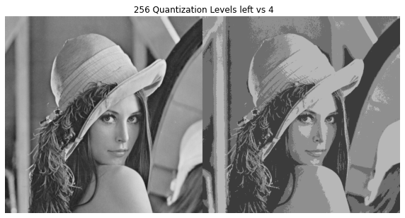
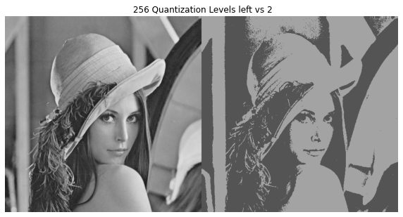
So quantization affect we can see the in pil image. We can do it opencv image manually.
Color channel
PIL
We can individually see each channel image using split funciton
red, green, blue = pil_image.split()
Now we have the varialbe (red, green, blue) which have the image of each channel separately.
Let’s see each channel side by side to compare it
get_concat_h(red, blue)

get_concat_h(red, green)

Actually it is better when we can see the color image and all channel image together. So following function will help us in this manner.
def concat_channel(red,
                   green,
                   blue):
    """
    Args:
        red ([type]): [description]
        green ([type]): [description]
        blue ([type]): [description]
    """
    im = Image.new('RGB', (red.width, red.height + green.height + blue.height))
    im.paste(red,(0,0))
    im.paste(green,(0,red.height))
    im.paste(blue,(0,red.height + green.height))
    return im
Let’s see whether our function works or not
fig, ax = plt.subplots(nrows=1, ncols=2, figsize=(10, 20))
axes = ax.ravel()
axes[0].imshow(pil_image)
axes[0].axis('off')
axes[0].set_title('3 Channel image')
axes[1].imshow(concat_channel(red, green, blue))
axes[1].axis('off')
axes[1].set_title('red channel(top), blue channel(bottom)');

Opencv
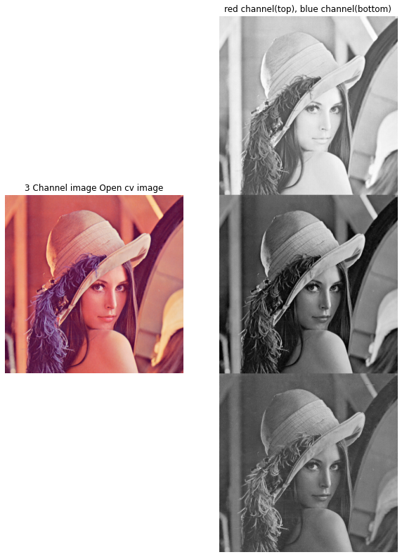
So we can do same thing with open cv image Previously we converted open cv imge from bgr to rgb image, so first channel is red, then green and after that blue image
red_cv, green_cv, blue_cv = new_cv_image[:, :, 0],  new_cv_image[:, :, 1], new_cv_image[:, :, 2]


fig, ax = plt.subplots(nrows=1, ncols=2, figsize=(10, 20))
axes = ax.ravel()
axes[0].imshow(new_cv_image)
axes[0].axis('off')
axes[0].set_title('3 Channel image Open cv image')
axes[1].imshow(cv2.vconcat([red_cv, green_cv, blue_cv]), cmap='gray')
axes[1].axis('off')
axes[1].set_title('red channel(top), blue channel(bottom)');
PIL Images to numpy array
import numpy as np
np.asarray generally manipualte images, but normally we would like to create a copy of the image and then do whatever we want to do with it. In this case np.array will help. In case of np.array it creates a copy of the image.
array = np.array(pil_image)
array.shape
(512, 512, 3)
array.max(), array.min()
(255, 3)
array[0, 0]
array([226, 137, 125], dtype=uint8)
Indexing
PIL
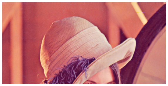
So here we can tell we want to see upto specific rows of data. and then all columns (means whole image in column axis), and all the channels
row_num = 256
show_image(array[0:row_num, :, :])
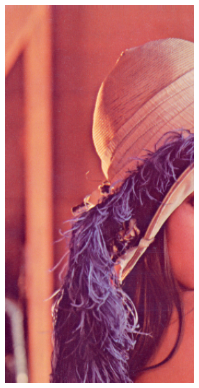
We can do same for specific columns
column_num = 256
show_image(array[:, 0: column_num, :])
We can reassign another variable to the image using
copymethod
A = array.copy()
show_image(A)

If we do not use
copymethod, the location of memory will be same
B = A
# We are assigning every value to zero to A image, that means A will be a dark image, but we don't change the B image
A[:,:,:] = 0
# let see the B image
show_image(B)

As we didnot use copy method, therefore same memory location. As a result manipulating A is affecting the B image
We actually can see the each channel image will color, if we want to see the red portion. we need to put the channel iamge to zero
Red image
red_image = array.copy()
red_image[:,:,1] = 0
red_image[:,:,2] = 0
show_image(red_image)

### Green image
green_image = array.copy()
green_image[:, :, 0] = 0
green_image[:, :, 2] = 0
show_image(green_image)

# blue image
blue_image = array.copy()
blue_image[:, :, 0] = 0
blue_image[:, :, 1] = 0
show_image(blue_image)

As normally in opencv the images are loaded as numpy array, so same indexing and color images visualization functionality we can use also for opencv images.
References
-
Images are taken from here
-
Overall this is the classnote of coursera course Introduction of Computer Vision and Image Processing